Modeling S&P 500 Using GARCH¶

In financial markets, predicting the direction of a stock price is incredibly difficult. However, predicting its volatility—how much the price is likely to fluctuate—is often more achievable and just as important for managing risk. This project will walk you through an end-to-end workflow for modeling the volatility of the S&P 500 index using a GARCH (Generalized Autoregressive Conditional Heteroskedasticity) model.

1. Data Acquisition and Preparation¶

Our first step is to acquire historical data for the S\&P 500 index (^GSPC) using the yfinance library. We'll focus on the daily 'Close' price from early 2015 to late 2023.

ticker = '^GSPC'
period1 = dt.datetime(2015, 1, 1)
period2 = dt.datetime(2023, 9, 22)
interval = '1d' # 1d, 1m

SP_500 = yf.download(ticker, start=period1, end=period2, interval=interval, progress=False)
SP_500 = SP_500.reset_index()

df=SP_500[["Date","Close"]]
df["unique_id"]="1"
df.columns=["ds", "y", "unique_id"]
StatsForecast.plot(df)

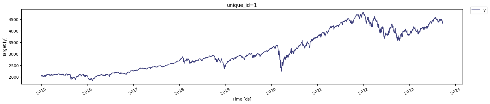
The statsforecast library requires the data to be in a specific format with columns named ds (for the date), y (for the value we're analyzing), and unique_id (to identify the time series). We rename our columns accordingly to prepare for modeling.

2. Analyzing the Raw Price Series¶

Before we can model volatility, we need to understand the characteristics of our data. Most statistical models, including those for volatility, assume the data is stationary. We can use the Augmented Dickey-Fuller (ADF) test to check for stationarity.

def Augmented_Dickey_Fuller_Test_func(series , column_name):
    print (f'Dickey-Fuller test results for columns: {column_name}')
    dftest = adfuller(series, autolag='AIC')
    dfoutput = pd.Series(dftest[0:4], index=['Test Statistic','p-value','No Lags Used','Number of observations used'])
    for key,value in dftest[4].items():
       dfoutput['Critical Value (%s)'%key] = value
    print (dfoutput)
    if dftest[1] <= 0.05:
        print("Conclusion:====>")
        print("Reject the null hypothesis")
        print("The data is stationary")
    else:
        print("Conclusion:====>")
        print("The null hypothesis cannot be rejected")
        print("The data is not stationary")


Augmented_Dickey_Fuller_Test_func(df["y"],'S&P500')

Interpreting the ADF Test Results

When we run the ADF test on the raw S\&P 500 closing prices, the p-value will be significantly greater than 0.05. This means we cannot reject the null hypothesis, leading to the conclusion that the raw price data is not stationary. It has a clear trend, making it unsuitable for direct modeling.

3. Transforming Data to Returns¶

To address the non-stationarity, we'll transform the price series into a series of daily returns. Returns are stationary and represent the percentage change in price from one day to the next.

df['return'] = 100 * df["y"].pct_change()
df.dropna(inplace=True, how='any')
df['sq_return'] = df["return"].mul(df["return"])

# visualizing the time series

base = alt.Chart(df).mark_line().encode(
    x='ds',
    # y='return',
).properties(
    width=800,
    height=400,
    # title="SP500 Return Chart"
)
return_chart = base.encode(
    y='return'
).properties(
    title="SP500 Return Chart"
)
sq_return_chart = base.encode(
    y='sq_return'
).properties(
    title="SP500 Squared Return Chart"
)

(return_chart | sq_return_chart).properties(
    title="SP500 Return and Squared Return Chart"
)

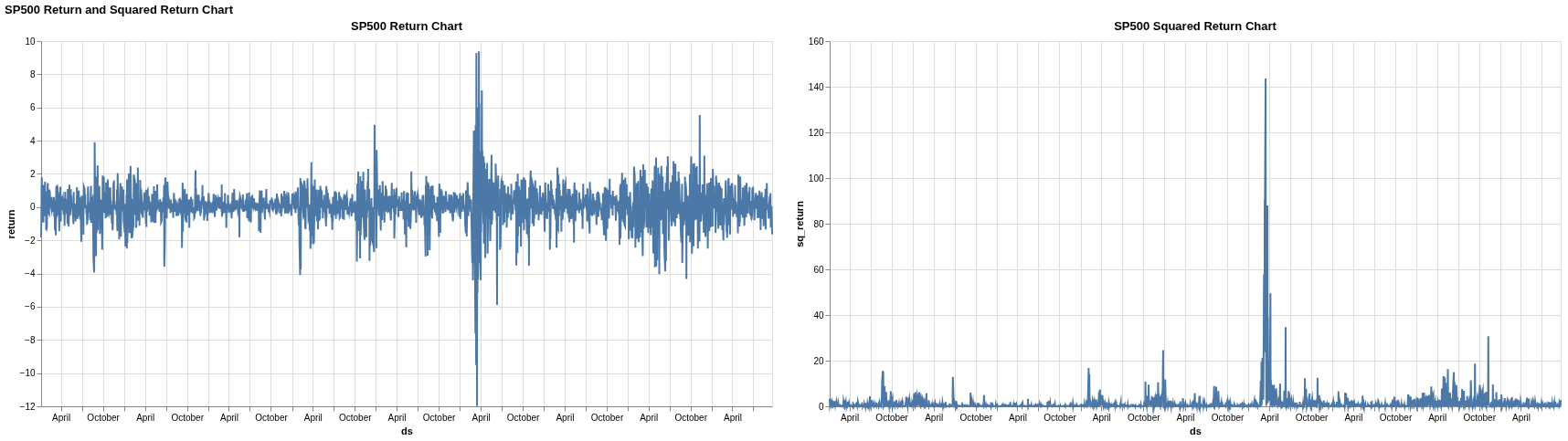
We also calculate the squared returns, as this is often used as a proxy for financial variance or volatility. The visualization of the returns and squared returns reveals a key characteristic of financial data known as volatility clustering. Notice how periods of high fluctuation are clumped together, followed by periods of relative calm. This is precisely the phenomenon that GARCH models are designed to capture.

4. Checking for Autocorrelation¶

Next, we use the Ljung-Box test to check if there is significant autocorrelation in our returns data. Autocorrelation means that past values are correlated with future values.

ljung_res = acorr_ljungbox(df["return"], lags= 40, boxpierce=True)

# ln_pvalue < 0.05 ? reject null hypotheses i.e. no autocorrelation
ljung_res.head()


df=df[["ds","unique_id","return"]]
df.columns=["ds", "unique_id", "y"]
train = df[df.ds<='2023-05-31'] # Let's forecast the last 30 days
test = df[df.ds>'2023-05-31']
train.shape, test.shape

Interpreting the Ljung-Box Test Results

The test results will show very small p-values <0.05 for our returns data. This leads us to reject the null hypothesis of no autocorrelation, confirming that the returns are indeed correlated with their past values. This is another signal that a time-dependent model like GARCH is appropriate.

5. Model Selection with Cross-Validation¶

A GARCH model is defined by two parameters, p and q, which represent the number of past squared returns and past variances to include in the model, respectively. To find the best combination of (p,q), we use cross-validation.

StatsForecast's cross_validation function automates this process by creating multiple "windows" of training data and testing how well different GARCH models perform at forecasting. We evaluate the models using the Root Mean Squared Error (RMSE), with the goal of finding the model order that produces the lowest average error.

season_length = 7 # Dayly data
horizon = len(test) # number of predictions biasadj=True, include_drift=True,

models = [GARCH(1,1),
          GARCH(1,2),
          GARCH(2,2),
          GARCH(2,1),
          GARCH(3,1),
          GARCH(3,2),
          GARCH(3,3),
          GARCH(1,3),
          GARCH(2,3)]

sf = StatsForecast(
    models=models,
    freq='C', # custom business day frequency
)

crossvalidation_df = sf.cross_validation(df=train,
                                         h=horizon,
                                         step_size=6,
                                         n_windows=5)

print(crossvalidation_df)


evals = evaluate(crossvalidation_df.drop(columns='cutoff'), metrics=[rmse], agg_fn='mean')
print(evals)

Based on the cross-validation results, the GARCH(1,1) model is often a strong performer for financial data, so we'll select that for our final model.

6. Fitting and Forecasting¶

Now, we fit our chosen GARCH(1,1) model to the training dataset and use it to forecast volatility for the hold-out test period.

season_length = 7 
horizon = len(test) 
models = [GARCH(1,1)]

sf = StatsForecast(models=models,
                   freq='C', 
                  )
sf.fit(df=train)

StatsForecast(models=[GARCH(1,1)], freq='C')

result=sf.fitted_[0,0].model_
display(result)

residual=pd.DataFrame(result.get("actual_residuals"), columns=["residual Model"])
display(residual)


Y_hat = sf.forecast(df=train, h=horizon, fitted=True, level=[95])
display(Y_hat.head())
values=sf.forecast_fitted_values()
display(values.head())
sf.plot(train, Y_hat.merge(test), max_insample_length=200)


forecast_df = sf.predict(h=horizon, level=[80,95])
sf.plot(train, test.merge(forecast_df), level=[80, 95], max_insample_length=200)

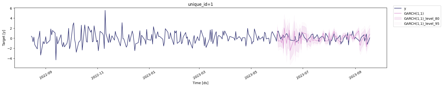
Predictions Plot — Predicted Returns and the Intervals

The plots generated by StatsForecast allow us to visually inspect how well our model's predictions align with the actual returns in the test set. The shaded regions represent the 80% and 95% prediction intervals, giving us a probabilistic range for our forecasts.

7. Final Model Evaluation¶

Finally, we quantitatively evaluate the model's performance on the test set using a variety of metrics.

evaluate(
    test.merge(Y_hat),
    metrics=[mae, mape, partial(mase, seasonality=season_length), rmse, smape],
    train_df=train,
)

Metrics like Mean Absolute Error (MAE) and Root Mean Squared Error (RMSE) tell us the average magnitude of our forecast errors in the same units as the original data (daily returns). The Mean Absolute Percentage Error (MAPE) gives us a sense of the error in percentage terms, which is often easier to interpret. This final evaluation gives us a concrete measure of how well our GARCH model can predict the volatility of the S&P 500.