Foundations of Time Series Analysis¶

The Nature of Time-Ordered Data¶

In business analytics, we encounter two primary types of datasets. The first is cross-sectional data, where the order of observations is not important. For example, when performing customer segmentation, each row represents a different customer, and shuffling the rows does not change the analytical outcome.

The second type is time series data, where observations are recorded sequentially over time. Examples include quarterly company earnings, daily website traffic, or minute-by-minute stock prices. In this context, the sequence is critical; the core assumption is that past values hold information that can help explain or forecast future values. Shuffling the data would destroy these vital temporal patterns. This lesson focuses exclusively on this second type of data.

Fundamental Concepts for Analyzing a Series¶

Before analyzing time series data, it's essential to understand a few key concepts that form the basis of many techniques. These concepts define how we "view" and transform the data to uncover insights.

Window

A window is a selection or "slice" of data points of a fixed size from a time series. Imagine you have daily sales data for a year. A window could be a seven-day period. This window can be moved across the data to perform calculations on small, sequential segments.

Fixed Window: A single block of time (e.g., analyzing data for only the first quarter).
Rolling Window: This is a more common and powerful concept where the window "slides" or "rolls" across the time series. For each step forward in time, the window moves one period, a new observation enters the window, and the oldest observation leaves.

Moving Average

A moving average is a practical application of a rolling window. It's a technique used to smooth out short-term fluctuations or "noise" in a time series, helping to reveal the underlying trend.

It is calculated by averaging the data points within a rolling window as it moves through the series. The "width" of the window (e.g., 7 days, 30 days) is a critical parameter.

Smaller Window Width (e.g., a 10-day moving average): More responsive to recent changes but less smooth.
Larger Window Width (e.g., a 90-day moving average): Produces a smoother line that highlights the long-term trend but is slower to react to new information.

Lag

A lag refers to a past value in a time series. A lag of 1 (t-1) for a daily series is the value from the previous day. A lag of 12 (t-12) for a monthly series is the value from the same month one year prior. The concept of a lag is fundamental to understanding how a series relates to its own past, a property known as autocorrelation, which will be covered in the next section of the lesson.

Structural Components of a Time Series¶

Most time series can be conceptually broken down into several underlying components that describe their behavior. The primary goal of exploratory analysis is to identify and understand these components, as they are key to selecting an appropriate forecasting model.

Trend 📈¶

The trend represents the long-term, underlying direction of the data, ignoring the short-term ups and downs. It reflects the persistent, long-run growth or decline of the series. For example, a company's annual revenue might show a consistent upward trend over a decade, even with some variability in quarterly earnings. Identifying the trend is crucial for long-range planning and forecasting.

Seasonality 📅¶

Seasonality refers to predictable, repeating patterns or fluctuations that occur at fixed intervals of time. These patterns are tied to a calendar, such as the day of the week, the month, or a quarter. A classic example is the surge in retail sales every fourth quarter due to holiday shopping. Recognizing seasonality is key for inventory management, staffing, and short-term forecasting.

Volatility ⚡¶

Volatility describes the magnitude of random, unpredictable fluctuations in the data. It's a measure of how much the series tends to vary over time. While all series have some randomness, financial data like stock prices are often characterized by periods of high volatility (large, rapid price swings) and low volatility (relative calm). Understanding volatility is critical for risk assessment and financial modeling.

Stationarity ⚖️¶

A time series is stationary if its statistical properties—specifically its mean, variance, and autocorrelation—are all constant over time. In simpler terms, a stationary series is one whose fundamental behavior doesn't change with time. A series with a clear trend or seasonality is, by definition, non-stationary because its mean or cyclical patterns change over time.

The reason stationarity is so important is that many powerful time series forecasting models (like ARIMA models) are designed to work on stationary data. These models assume that the process generating the data is stable, making it possible to model and predict future values. To use these models on non-stationary data, we must first apply transformations to make the series stationary. A common method to remove a trend is differencing, which we will explore in later modules.

Before we can effectively apply analytical concepts like moving averages, we must first ensure our data is clean, complete, and uniformly structured. Real-world time series data is rarely perfect. The following section addresses the most common data preparation tasks that are specific to time-ordered data.

Common Data Wrangling Tasks for Time Series¶

While standard data cleaning is always necessary, time series data presents several unique challenges. The methods used to address these issues must respect the temporal ordering of the data to avoid introducing bias or error.

Handling Missing Data¶

In a standard dataset, you might fill missing values with the mean or median of the entire column. With time series data, this is often a poor choice as it ignores the temporal structure. More appropriate methods include:

Forward Fill (ffill) or Backward Fill (bfill): This propagates the last known observation forward or the next known observation backward. It's a simple method, useful when observations don't change rapidly.
Interpolation: This involves filling missing values by estimating them based on neighboring points. Linear interpolation, which assumes a straight line between two points, is common. More complex methods like polynomial or spline interpolation can also be used.
Seasonal Adjustment: For data with strong seasonality, missing values can be imputed using the value from a previous season (e.g., the same month in the prior year).

import polars as pl
from datetime import date

df_missing = pl.DataFrame({
    "date": [dt.date(2024, 1, 1), dt.date(2024, 1, 2), dt.date(2024, 1, 3)],
    "value": [10, None, 15]
})

df = (
    df_missing
    .with_columns(
        pl.col("value")
        .fill_null(strategy="forward")
        .alias("value_forward")
        )
    .with_columns(
        pl.col("value")
        .fill_null(strategy="backward")
        .alias("value_backward")
    )
    .with_columns(
        pl.col("value")
        .fill_null(strategy="mean")
        .alias("value_mean")
    )
)
print(df)

Resampling¶

Resampling is the process of changing the data's frequency. It's a common and powerful technique:

Downsampling: Aggregating data from a high frequency to a lower frequency (e.g., from daily to monthly). This is used to smooth out noise and identify long-term trends. You must choose an appropriate aggregation method, such as mean(), sum(), or last().
Upsampling: Increasing the frequency of the data (e.g., from monthly to daily). This is less common and requires careful application of an imputation method (like forward fill or interpolation) to fill in the newly created gaps.

# Example DataFrame with daily data
df_daily = pl.DataFrame({
    "date": pl.date_range(date(2024, 1, 1), date(2024, 2, 15), "1d", eager=True),
    "sales": range(46)
})

# Downsample to monthly average sales
df_monthly = df_daily.group_by_dynamic(
    "date", every="1mo"
).agg(
    pl.col("sales").mean().alias("average_sales")
)
print(df_monthly)

Dealing with Irregular Timestamps¶

Not all time series are recorded at perfect intervals. Financial transaction data or sensor readings, for example, may arrive at irregular times. Many statistical models assume a fixed frequency. To handle this, you may need to regularize the time series by creating a fixed-interval time index and mapping the irregular observations to this new index, using an appropriate aggregation or imputation method to fill the gaps.

Timezone Localization and Conversion¶

Data collected from different geographic locations or systems may have different or nonexistent timezone information. It is critical to standardize all timestamps to a single timezone, typically Coordinated Universal Time (UTC), to ensure that calculations and sequences are correct. This process involves:

Localization: Assigning a timezone to "naive" timestamps that lack this information.
Conversion: Converting "aware" timestamps from one timezone to another.

Code Demo: EDA with Stock Prices¶

Now, let's apply these concepts using Polars and Altair to analyze daily stock price data for a company like Google (GOOG).

First, we load the data and ensure the Date column is correctly formatted as a datetime object.

import polars as pl
import altair as alt

# This example assumes you have a CSV with stock data
# You can often download this from financial sites like Yahoo Finance
file_path = 'path/to/your/GOOG.csv'
df = pl.read_csv(file_path)

# Ensure the Date column is a datetime object for time series operations
df = df.with_columns(
    pl.col("Date").str.to_date(format="%Y-%m-%d")
)

# Plot the daily closing price
base = alt.Chart(df).encode(x='Date:T')

closing_price = base.mark_line().encode(
    y=alt.Y('Close:Q', title='Closing Price (USD)')
).properties(
    title='Google (GOOG) Daily Stock Price'
)

closing_price.display()

The raw price data is volatile. To better see the trend, we can calculate and plot moving averages using a rolling window. Notice how we explicitly define the window width (window_size).

# Calculate 30-day and 90-day moving averages
df_with_ma = df.with_columns(
    pl.col("Close").rolling_mean(window_size=30).alias("ma_30_day"),
    pl.col("Close").rolling_mean(window_size=90).alias("ma_90_day")
)

# Create layers for the moving averages
ma_30 = base.mark_line(color='orange').encode(
    y='ma_30_day:Q'
)

ma_90 = base.mark_line(color='red').encode(
    y='ma_90_day:Q'
)

# Combine the original price plot with the moving average plots
(closing_price + ma_30 + ma_90).interactive().display()

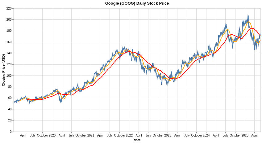
GOOG Stock Price: Time Series Visualized — Comparing 30 and 90 day moving averages with daily price changes.

In the combined chart, you can clearly see how the 30-day moving average (orange) follows the price more closely, while the 90-day moving average (red) provides a much smoother line, making the longer-term trend easier to discern. This demonstrates the practical effect of choosing different window widths for analysis.