Workflow in Action

Workflow in Action¶

In this we will translate the six-step theoretical workflow into a practical, end-to-end coding exercise. You will train, predict with, and evaluate your first machine learning model using a Iris dataset, a classic toy dataset tht's very useful for learning various topics in machine learning.

Objective: Apply the complete modeling workflow to the Iris dataset using scikit-learn and develop familiarity with scikit-learn's estimator API.

Setup: Importing Libraries¶

First, we import the necessary libraries. We need Polars for data handling and various modules from scikit-learn for loading the dataset, splitting the data, instantiating the model, and evaluating its performance.

import polars as pl
from sklearn.datasets import load_iris
from sklearn.model_selection import train_test_split
from sklearn.tree import DecisionTreeClassifier
from sklearn.metrics import accuracy_score

# For the bonus visualization
import matplotlib.pyplot as plt
from sklearn.tree import plot_tree

Step 1: Load & Prepare Data¶

We will use the classic Iris dataset, which is conveniently included with scikit-learn. Our first action is to load the data and convert it into a Polars DataFrame, which allows for easier inspection and manipulation. We then separate our features (X) from our target (y).

# Load the dataset from scikit-learn
iris_data = load_iris()

# Create a Polars DataFrame
# The data is in '.data' and column names in '.feature_names'
df = pl.DataFrame(
    data=iris_data.data,
    schema=iris_data.feature_names
).with_columns(
    # Add the target variable, which is in '.target'
    pl.Series(name="target", values=iris_data.target)
)

# Define our features (X) and target (y)
X = df.select(pl.exclude("target"))
y = df.select("target")

# Display the first 5 rows of the feature DataFrame
print("Features (X):")
print(X.head())

# Display the first 5 rows of the target DataFrame
print("\nTarget (y):")
print(y.head())

Step 2: Split the Data¶

Next, we partition the data into training and testing sets. This is a critical step to ensure an unbiased evaluation of our model. We will allocate 30% of the data for the test set and set a random_state to ensure that our split is reproducible every time the code is run.

X_train, X_test, y_train, y_test = train_test_split(
    X, y, test_size=0.3, random_state=42
)

# Verify the dimensions of the resulting datasets
print(f"Shape of X_train: {X_train.shape}")
print(f"Shape of X_test: {X_test.shape}")

You should see that X_train has 105 rows and X_test has 45 rows, corresponding to a 70/30 split of the original 150 rows.

Step 3: Instantiate the Model¶

We will now instantiate our DecisionTreeClassifier. To prevent the model from becoming overly complex, we will set the max_depth hyperparameter to 3. We also pass the random_state for reproducibility of the model's training process.

model = DecisionTreeClassifier(max_depth=3, random_state=42)
print(model)

Step 4: Train the Model¶

With our model instance created and our training data ready, we can execute the training step. We use the .fit() method on our training data (X_train and y_train).

model.fit(X_train, y_train)

After this cell runs, the model object is no longer an empty shell; it now contains the learned rules (parameters) from the Iris training data.

Step 5: Generate Predictions¶

Our model is now trained. We can use the .predict() method to generate predictions on the unseen data we held back in our test set (X_test).

# Generate predictions for the test set
predictions = model.predict(X_test)

# Display the first 10 predictions
print(predictions[:10])

Step 6: Evaluate Model Performance¶

This is the final step where we quantify the model's performance. We compare the predictions our model made against the actual ground truth labels in y_test using the accuracy_score metric.

# Calculate the accuracy of the model
accuracy = accuracy_score(y_test, predictions)

print(f"Model Accuracy on Test Set: {accuracy:.4f}")

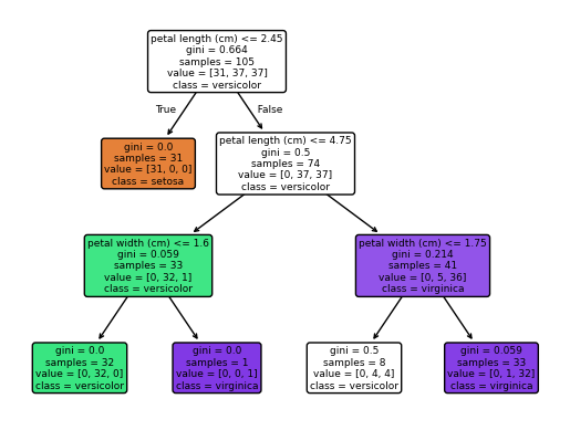
The accuracy score represents the proportion of correct classifications. An accuracy of 1.0 would mean a perfect score on the test set.

Visualizing the Model's Logic¶

A key advantage of the Decision Tree is its interpretability. We can visualize the rules the model learned during the .fit() step to understand exactly how it is making decisions.

# Set the figure size for better readability
plt.figure(figsize=(20, 10))

# Create the plot
plot_tree(
    model,
    feature_names=X.columns,
    class_names=iris_data.target_names,
    filled=True,
    rounded=True
)

# Display the plot
plt.show()

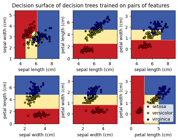
This visualization shows the flowchart that the model uses. Starting from the top (root) node, you can trace a path down the tree based on the feature values of a given flower to see how it arrives at a final classification (leaf node).

Iris: Decision Tree — Looking under the hood of a decision tree model

We can also visually explore to understand how different features contribute to how model performs and identify opportunities to simplify the model in the next iteration.

iris = load_iris()

# Parameters
n_classes = 3
plot_colors = "ryb"
plot_step = 0.02


for pairidx, pair in enumerate([[0, 1], [0, 2], [0, 3], [1, 2], [1, 3], [2, 3]]):
    # We only take the two corresponding features
    X = iris.data[:, pair]
    y = iris.target
    class_names = iris.target_names

    # Train
    clf = tree.DecisionTreeClassifier(max_depth=3, random_state=42).fit(X, y)

    # Plot the decision boundary
    ax = plt.subplot(2, 3, pairidx + 1)
    plt.tight_layout(h_pad=0.5, w_pad=0.5, pad=2.5)
    DecisionBoundaryDisplay.from_estimator(
        clf,
        X,
        cmap=plt.cm.RdYlBu,
        response_method="predict",
        ax=ax,
        xlabel=iris.feature_names[pair[0]],
        ylabel=iris.feature_names[pair[1]],
    )

    # Plot the training points
    for i, color in zip(range(n_classes), plot_colors):
        idx = np.asarray(y == i).nonzero()
        plt.scatter(
            X[idx, 0],
            X[idx, 1],
            c=color,
            label=iris.target_names[i],
            edgecolor="black",
            s=15,
        )

plt.suptitle("Decision surface of decision trees trained on pairs of features")
plt.legend(loc="lower right", borderpad=0, handletextpad=0)
_ = plt.axis("tight")